ENGR 3370: Controls
Characterization of a voith-schneider propeller
(A Collaboration with Victoria Coleman)
Overview
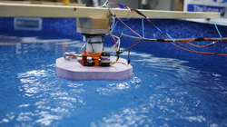
The Voith Schneider Propeller allows for maneuvering in tight spaces. However this advantage comes at a cost: the propeller is challenging to direct thrust in a specific direction. We created a six degree of freedom testing rig in order to calculate the thrust generated by the propeller and experimentally collected the values to derive the poles and zeros based on the time response of our system.
Introduction
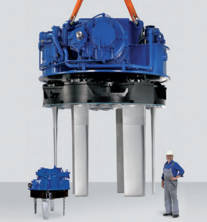
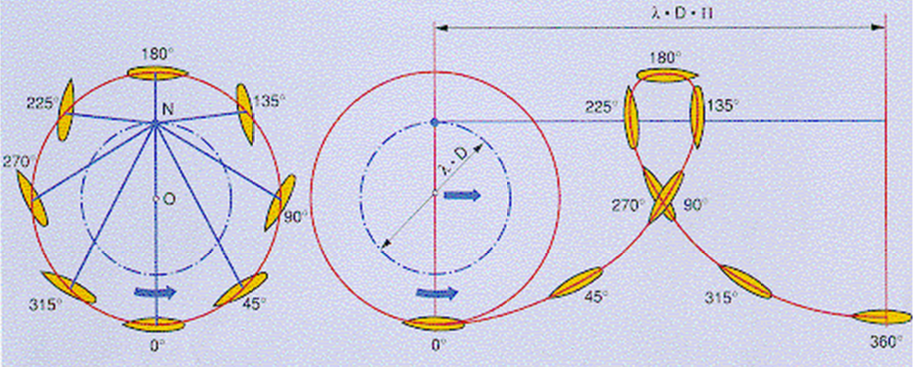
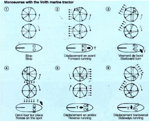
The Voith Schneider Propeller is a vertical variable pitch propeller system that allows for highly maneuverable watercraft due to its ability to apply thrust in any direction on the surface of the water. This system was designed in the 1920s and is still utilized today by naval craft, fire-fighting boats, and tugboat carriers. An example of what the propellers look like in real life are seen in figure 1. The blades are attached to a series of cams that allow their pitch to be controlled by a single pivot point at the top of the propeller. These blades are also mounted to a rotating cylinder which gives the initial velocity of the craft. Thrust is generated by the movement of the individual blades with respect to the water, while the thrust direction is determined by the relative phasing of the blades with respect to the disc. Thrust increases with the pitch of the blade. A more visual explanation of the cam linkage and change in thrust can be seen in figures 2 and 3.
|
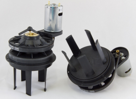
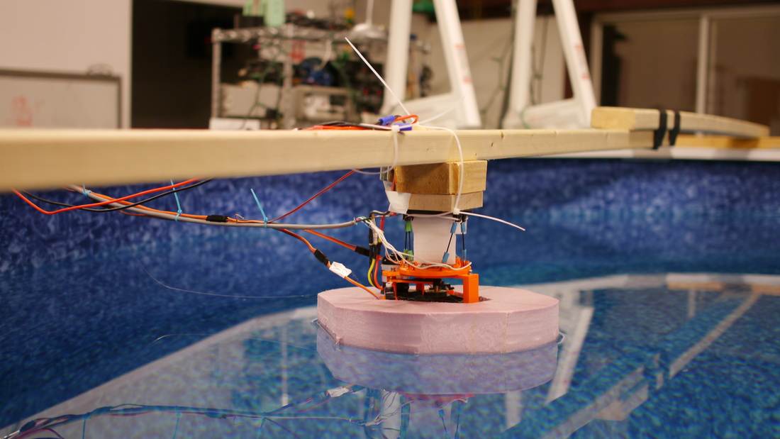
Our project focused on the challenges posed by a highly maneuverable vehicle based on the hobby-grade VSPs made by the German company, Graupner, as shown in figure 4. As this is a highly sensitive vehicle, we wanted to be able to map the correct position of the joysticks and derive the characteristics of the propeller in order to better control it. Originally we had wanted to mount two motors into a box so as to actually build a feedback loop with an IMU, however IMUs have inherent problems with drift. Another option was to have feedback through the ceiling-mounted camera above the large project building pool, however sending commands back to the vehicle meant that we would need to have wireless serial communication, which was not within the range of our price budget and would involve a fairly high level of complexity. Our final decision was to measure the thrust vector with a load cell and time the response from the time we sent the position command to the servos that controlled the position of the control linkage to when it finally peaked and stabilized at that specific thrust.
|
Our System
Sensor Implementation:
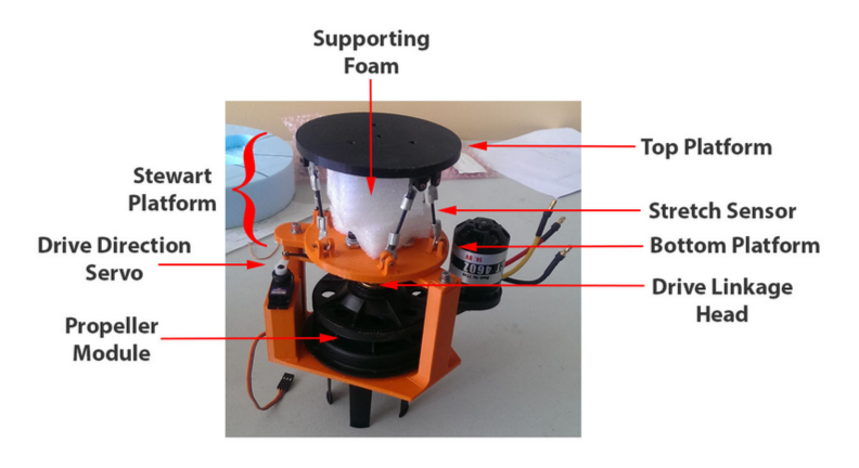
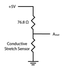
Each of the six variable resistance stretch sensors were a part of a simple voltage divider that was powered by the arduino and read by one of the analog in pins as shown in figure 8. For a sense of scale, the conductive stretch sensors had resistances of about 68-78 Ω when only barely taunt. Originally, a low-pass filter for each sensor with a critical frequency of about 20Hz was implemented, but was removed for simplicity. With more time, these filters should be replaced to decrease the noise of the system on a hardware level before smoothing on the software side. The top hooks of the platform were all connected and grounded from the arduino, and connections from the bottom hooks were fed back to be connected to the voltage divider.
To calibrate each sensor, we connected one end to 5 V and the other to an analog read port to measure the voltage across the sensor. We then hung two known weights (114.4 g and 318.5 g) in succession from the end of the sensor and recorded the length and voltage each time. We also measured the initial resting length of each sensor. With this information, we able to calculate the k constants of the rubber lengths (k = F/(X - Xo)) and the linear equation to map the voltage to length of the sensor. The documentation claims that the sensors have a linear characteristic, but experimentation showed that, while not completely true, it is a good representation when in the stretched state not close to the relaxed state. We originally collected resistance data on the sensors for various stretch lengths, so we could use the voltage divider equation to calculate the resistance of the sensor and then map it to length. By correlating the voltage to length instead, we made the system more accurate by having fewer steps for the error to compound.
With known geometry of the sensors, we could determine the force vectors for each sensor, map them to the origin, add them together, then project them on the 2D plane parallel to the plane of the stewart platform. Since the there is not much movement of the stewart platform (and even less change in the angle of the sensors relative to the platform), we assumed that the geometry was static.
Data Collection and Processing
To collect the data, we ran a script on the arduino that that controls the speed of the motor and the xy position of the control linkage head. The xy position was changed every 10 seconds to allow the transient behavior to fully dissipate before a new position command was sent. There were 8 positions the system cycles through which were the permutations of the 3 positions for each servo (Max, Min, and Neutral). The arduino also collected the sensor data and processed it to send an array of the magnitudes of the forces experienced by the sensors along with the command sent to the linkage head to the computer. A python script on the computer connected to the arduino received, timestamped, and saved this information to a .csv file on the computer. While we did not do data processing in real time, because we saved the raw data, we can try several processing methods on a set of data post-collection. Another python script does simple averaging of the data (exponential rolling average with a weight for the current data of less than .5) and then does the mapping and combining to generate a net force.
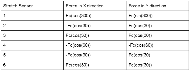
From the CAD model, we determined that the angle the sensor was mounted at was 30 degrees relative to the original coordinate frame set up that the sensor mount positions followed. The angle from that coordinate frame to the new coordinate frame in which we were comparing forces was 30 degrees, hence the forces felt by each stretch sensor could be found by the following (where Fc = Calculated Force from the stretch sensor data and all angles are in degrees):
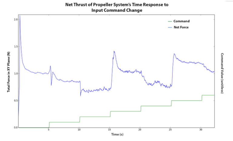
We then plotted the magnitude of the net thrust from the propeller system against time. We also plotted the current command to the motor so we could tell when a change happened because we wanted to analyze the response to a change in command.
Data Analysis
After running our experiment of plotting the thrust magnitude of the propeller system against time for a variety of positions of the drive linkage head, we produced the following plot as shown in figure 9.
Data Analysis
After running our experiment of plotting the thrust magnitude of the propeller system against time for a variety of positions of the drive linkage head, we produced the following plot as shown in figure 9.
The cleanest and seemingly most characteristic response time of the system occurred when the command changed at about 15 seconds. A zoom-in of this time response can be seen in figure 10. The system displays second order characteristics, and we were able to calculate values for the percent peak overshoot, time to peak, 1% settling time (how long it takes to get within and stay within 1% of the final settled value), and 10-90% rise time. The results are listed below:
Peak overshoot = 102.3%
Time to peak = .69s
10-90% rise time = .18s
The 1% settling time could not be precisely calculated since the test did not give enough time for the system to completely settle before exciting the next time response. It is guessed that it is around 5-6 seconds. As a result of this issue, the calculated settling value of .2391 (calculated from average of the last second of the recorded response time) will be a little off. With these values, we should be able to calculate the characteristic equation, which is in the form:
Knowing that Peak overshoot = exp(-πζ / (sqrt(1-ζ^2))) exactly, we can solve that equation for ζ, the damping coefficient. Since our peak overshoot is above 1, it is giving us a negative damping coefficient, so another method might need to be used for this system. We can also solve for ω by knowing the time to peak = π / (ωsqrt(1-ζ^2)). Our guess was that the values were not quite accurate from our experiment and since we got a negative number for zeta we figured we would just leave our data as is for future calculations of poles and zeros.
Unfortunately, this is our only clean graph. The waterproofing failed and at specific thrust directions, the foam flotation started filling with water. To fix this issue, we attempted to add more sealant and hot-glued the propeller system into the foam for a stronger mechanical attachment. The propeller system was accidentally glued in at a slight angle, still leaked, and gave noisy data. This could be attributed to the poor positioning of the propeller system and or the poor positioning of the brushless motor (interfered with the plastic mount at specific thrusts). The next fix we tried was to re-glue the motor with silicone aquarium sealant. However the system was still noisy, which we guess might be due to the small amount of sealant that got into the crevice of the rotating plate of the propeller system which might be causing some sticking. Another hypothesis is that because of the low current passing through our sensors, the resistance of the copper highly influenced our measurements and it is quite possible that the exposure to water, although not obvious, could have caused calcium build-up on our contacts between the stretch sensors, which could have created greater resistance and affected our measurements. Adding back in low-pass filters could help with the visible vibrations that are now evident in the sensor since the improved waterproofing. Another potential problem lies within the mount itself as it is not as rigid as we had hoped and flexes quite a bit when the servos move the linkages. Since the servos are coupled at right angles to each other, we noticed that there is a limited range in which the servos can actually move through since they move in arcs. A solution to that would require either a flexible linkage or a design of a stacked ball linkage that would allow both servos to move the control linkage without being forced to move in a planar motion, similar to figure 11, except that the double ball linkage would be on the control linkage as opposed to the servos.
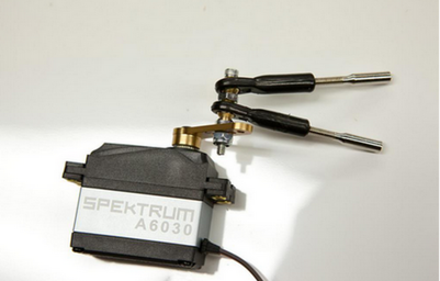
Figure 11. An example of a stacked double-ball linkage, which might be a system we have to look at for improving the controllability of the mechanical system. Both servos are rigidly coupled at 90 degrees, however since the servos themselves move in a circular fashion, there is a limited range of how far the control linkage can move and consequently we cannot send thrust vectors in all directions. This stacked double-ball linkage would be mounted onto the control linkage, not the servo, but would allow for each servo to control the linkage independently and increase the range.
Results
From our transfer function, we derived time-based constants such as (rise time, settling time, peak overshoot, steady-state-error). From here we calculated the poles and zeros necessary for our system to be stable.
Conclusion
There are lots of applications for our data. Now that we have characterized our system we can approximate its behavior and ensure stability for future vehicles. We also have the data for the mapping of servo commands to thrust direction and can apply our findings to a two-motor system, which will hopefully be able to be joystick controlled from this data.
References
D. Jurgens, M. Palm, “Voith Schneider Propeller - An Efficient Propulsion System for DP Controlled Vessels,” Dynamic Positioning Conference, Marine Technology Society, Oct. 2009.
http://www.dynamic-positioning.com/dp2009/thrusters_palm.pdf
D. Jurgens, M. Palm. “Voith Water Tractor -- Improved Manoeuvrability and Seakeeping Behaviour,” Tugnology, 2009
http://towmasters.files.wordpress.com/2009/06/voithwatertractor.pdf
A. Sorensen, “Marine Control Systems: Propulsion and Motion Control of Ships and Ocean Structures,” Lecture Notes from the Norwegian University of Science and Technology, 2013.
http://www.dynamic-positioning.com/dp2009/thrusters_palm.pdf
“Voith Schneider Propeller,” Voith Turbo website.
http://www.voith.com/en/products-services/power-transmission/voith-schneider-propeller-10002html
